Plotting Brain Surfaces
Overview
This module provides a streamlined interface for visualizing brain surface data. It includes three core functions tailored for different anatomical scopes:
draw_cortex– cortical data (fsLR surfaces, Schaefer/Glasser atlases)Data could be both in vertex space or parcellated space, the function will map automatically
Medial wall will be automatically restored if the data lack
draw_subcortex_tian– subcortical data (Tian 2020 atlas)draw_sftian– combined cortical + subcortical visualization
Medial Wall Problem
Vertex-wise datasets often exclude the medial wall (the non-cortical connection between hemispheres). In the standard fsLR-32k space, a full surface mesh contains 64,984 vertices, but the real data is frequently restricted to the 54,984 cortical vertices that exclude the medial wall.
The data overlayed on the geometry file should have the same point size. Given the geometry file includes medial wall, your data should always include the medial wall with zero value or np.nan.
The draw_cortex function automatically handles this discrepancy. If your input data omits the medial wall, the function will detect and pad the data appropriately, allowing you to focus on visualization without manual preprocessing.
Cortical Surface Visualization
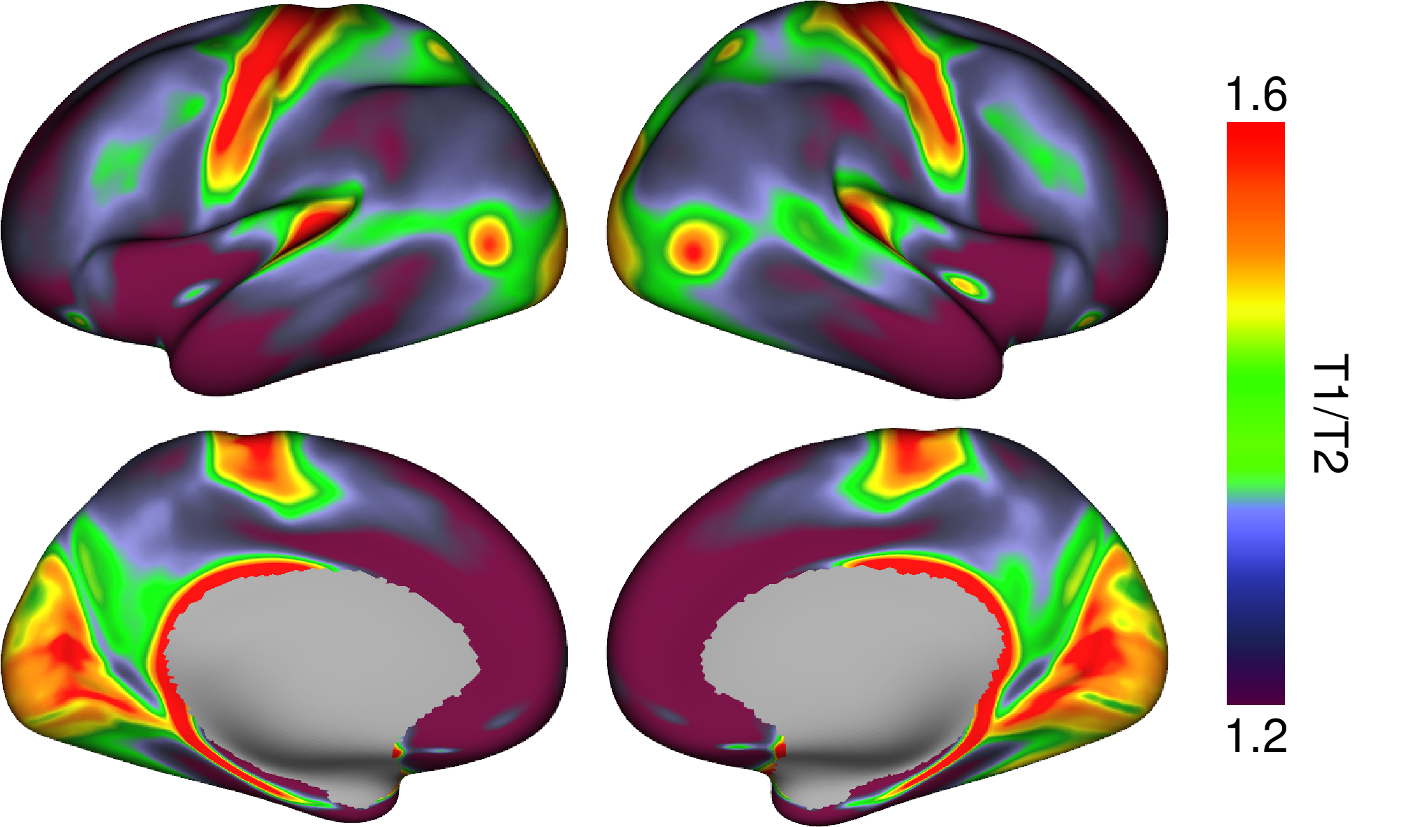
draw_cortex is used to render the cerebral cortex.
>>> from neurocat.plotting import draw_cortex as dc
>>> from neurocat import color

>>> dc(t1t2,
>>>    color.cmap.myelin(),
>>>    (1.2,1.6),
>>>    legend='T1/T2'
>>>   )
If your data is defined/calculated in parcellated (atlas) space, you do not need to manually map it to surface vertices. draw_cortex performs this conversion internally.
Common parcellations such as the Schaefer and Glasser atlases are supported internally; the function automatically identifies the atlas from the length of the input vector.
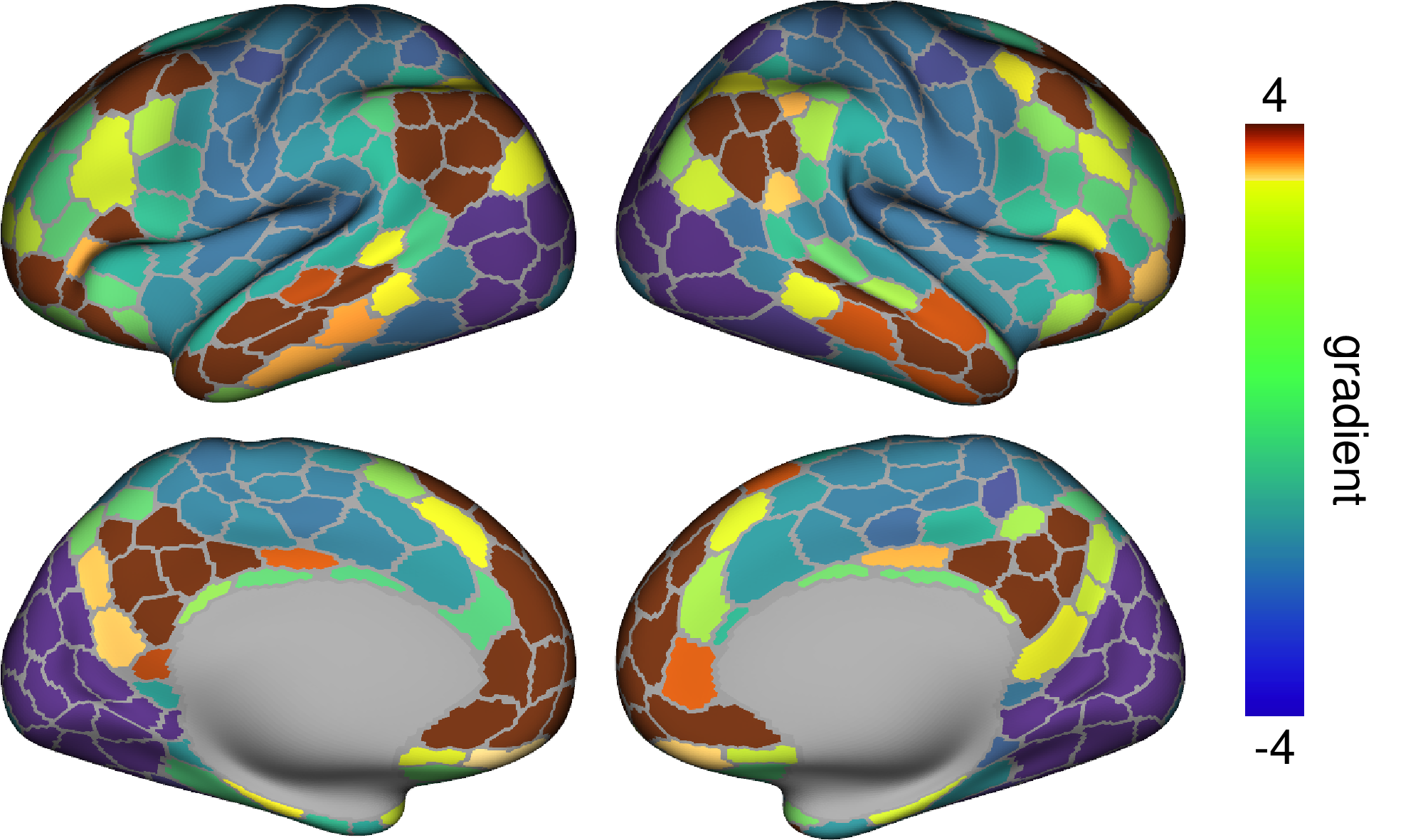
The following example computes the principal functional connectivity gradient using the Schaefer 400-parcel atlas and visualizes the result directly on the cortical surface.
>>> dc(fc_principal,
>>>    color.cmap.gradient(),
>>>    (-5,5),
>>>    legend='gradient'
>>>   )
Refer to the API of neurocat.plotting.draw_cortex() for all possible keywords.
Subcortical Visualization
draw_sftian enables simultaneous visualization of both cortical and subcortical structures. For cortical data, input should be parcellated using the Schaefer 400 or 1000 atlas; subcortical data should correspond to the Tian 2020 atlas. The combined input vector should therefore have a length of either 432 (Schaefer 400 + Tian) or 1030 (Schaefer 1000 + Tian).
Attention
The fsLR version of the Schaefer 1000 atlas is missing two labels due to the transformation from fsaverage6 to fsLR. For more details, see issue1, issue2, and issue3.
Note
Subcortical mesh files are provided by courtesy of Sidhant Chopra from their work. The meshes were reconstructed and smoothed using pyvista.
>>> from neurocat.plotting import draw_cortex as dc
>>> from neurocat import color

>>> dc(t1t2,
>>>    color.cmap.myelin(),
>>>    (1.2,1.6),
>>>    legend='T1/T2'
>>>   )
Refer to the API of neurocat.plotting.draw_sftian() for all possible keywords.